It is unfortunately all too common for many people performing data entry work to suffer from Fat Finger Syndrome. Imagine creating a detailed sales report for your company, handing it off to your executives, only to find out that Michael only had half of his usual sales for the month, because 50% of his entries were spelt Micheal instead of Michael. Poor Michael.
Ensuring that salesmen named Michael get their full month’s commission isn’t the only reason for creating a drop-down list though. Some spreadsheets are built to distribute to different people to log data with, whom of which may not be aware of what an example answer may be for any given column. Or you want to restrict the values in a column to a certain list of available options. Whatever the reason is, the solution is easy with only a few trivial steps!
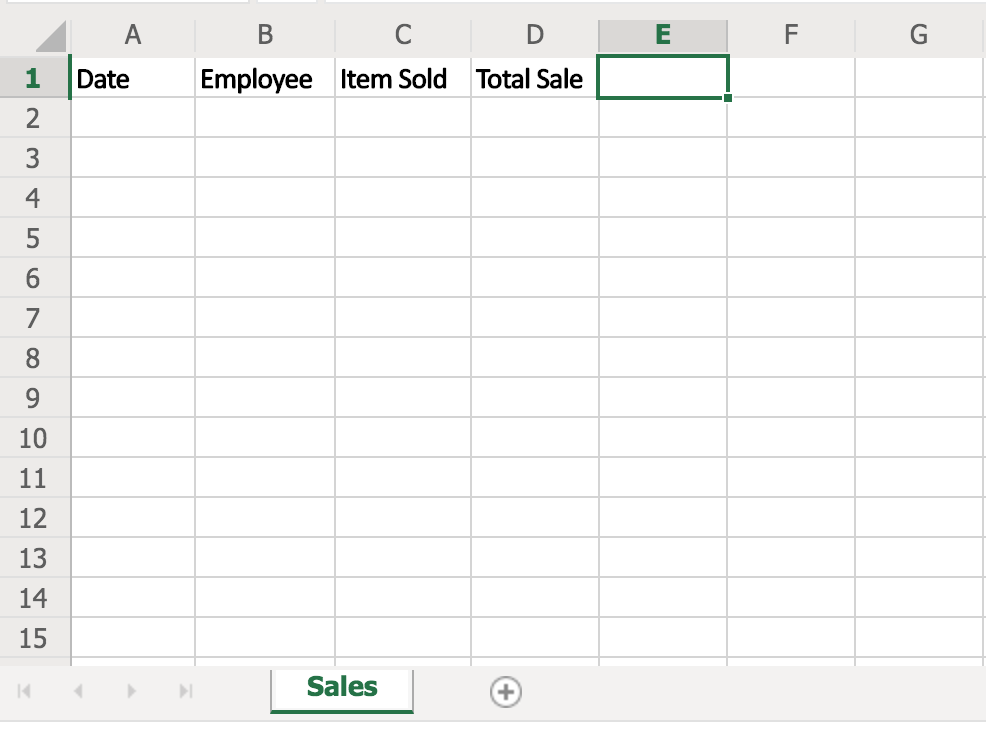
Before we actually create a list, we need a table to enter data in. For this example, let’s assume we’re keeping track of a sales record table and want to ensure that some of the columns provide a drop-down list to choose a value from. (More than likely you already have a table you need to add your drop down list to, so just jump to the next part)
Create lists in new separate tab
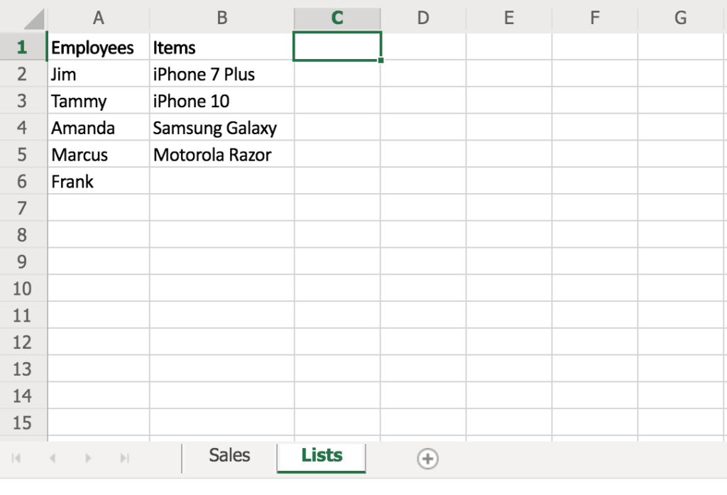
In order to create a drop down list, we will need to create the list range. For this, I like to keep a separate tab for all my drop down lists.
- Create new Tab
- Make your list(s)
- Pro Tip: if you have many lists, it makes it easier to add a header label to each list. Just make sure the header is not included in the data range, explained later
Add list range to Data Validation
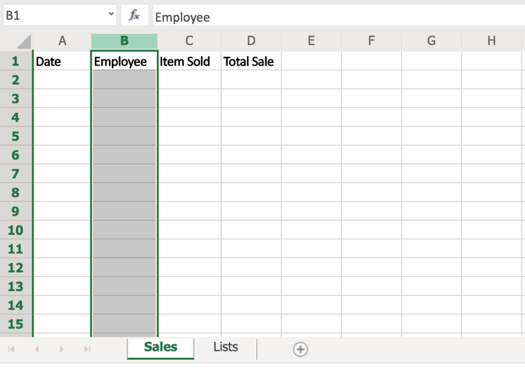
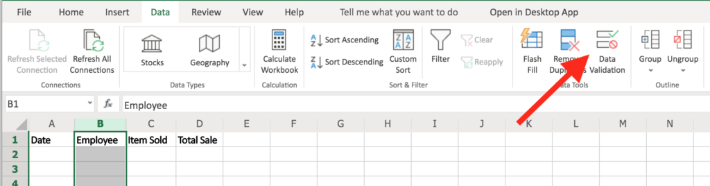
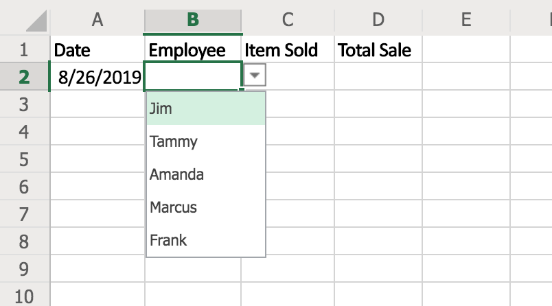
Now, back in your main Excel tab, click on the column header for the column you wish to add a drop down list for. In this example, we will be adding 2 drop down lists, one for Column B, and one for Column C.
- Click on the B Header Cell
- Click “Data” (top Navbar Menu)
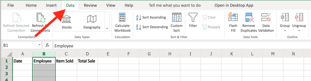
- Click “Data Validation” in Icon Sub-Menu
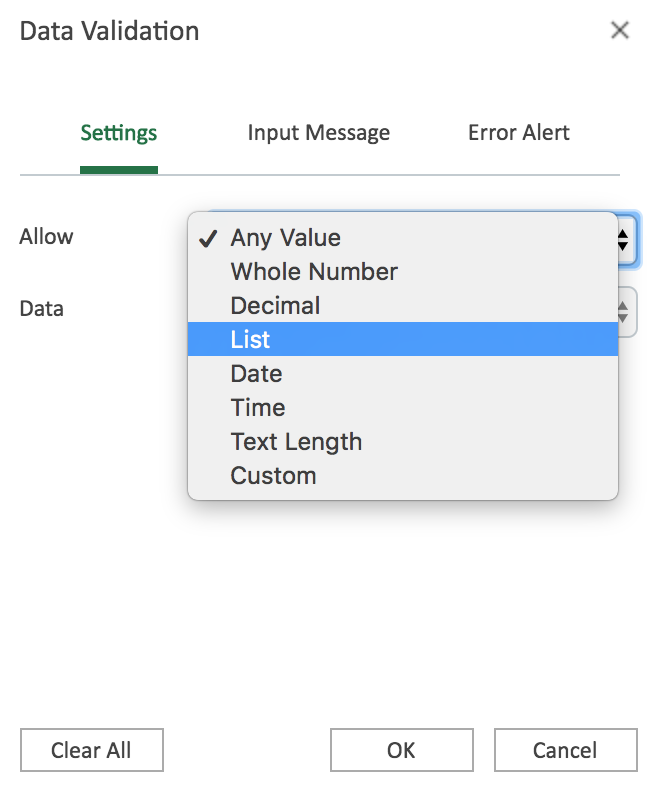
- In the “Allow” drop down menu, select “List”
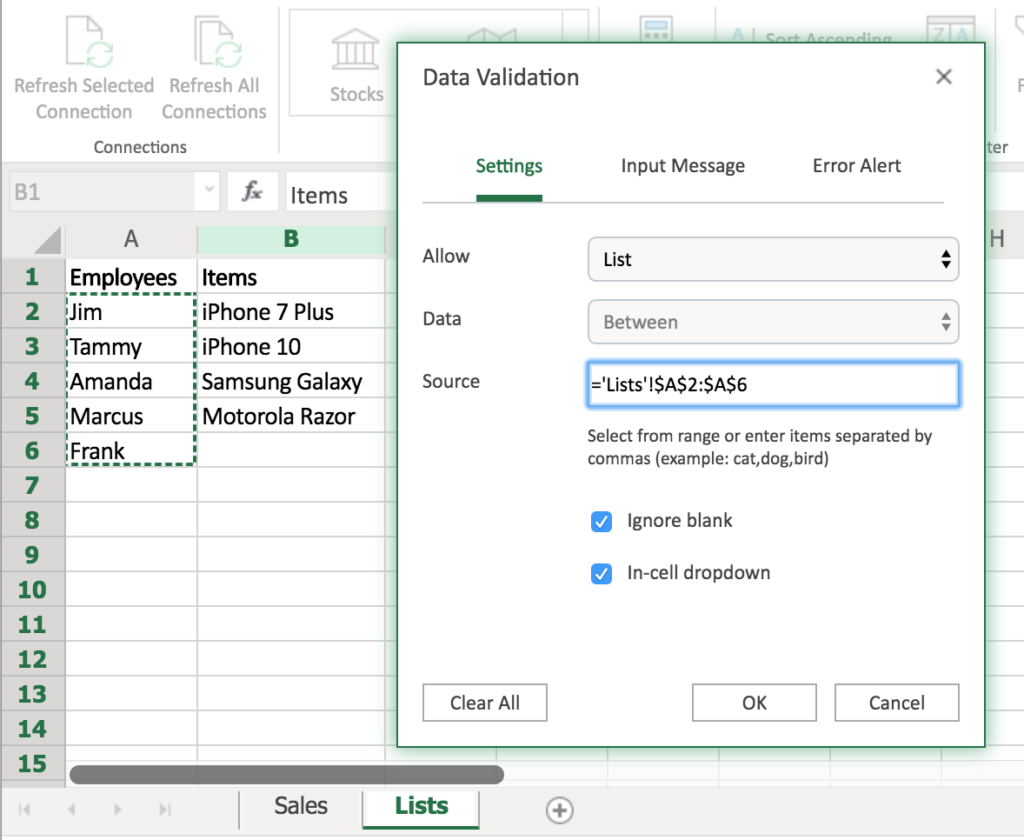
When you select “List” a new input field will display called Source. Click inside the Source input field, then find your list you want to use as the “Source” for this drop-down list.
In this case, we want to use our Employees list (A2 : A6) as the drop-down list for our Employees in Column B. So we will click inside the Source input field, then click back into our Lists tab, and click and drag from cell A2 to A6.
- Click inside Source input field
- Go to Lists tab
- Highlight cells A2, A3, A4, A5, and A6
- Press Enter
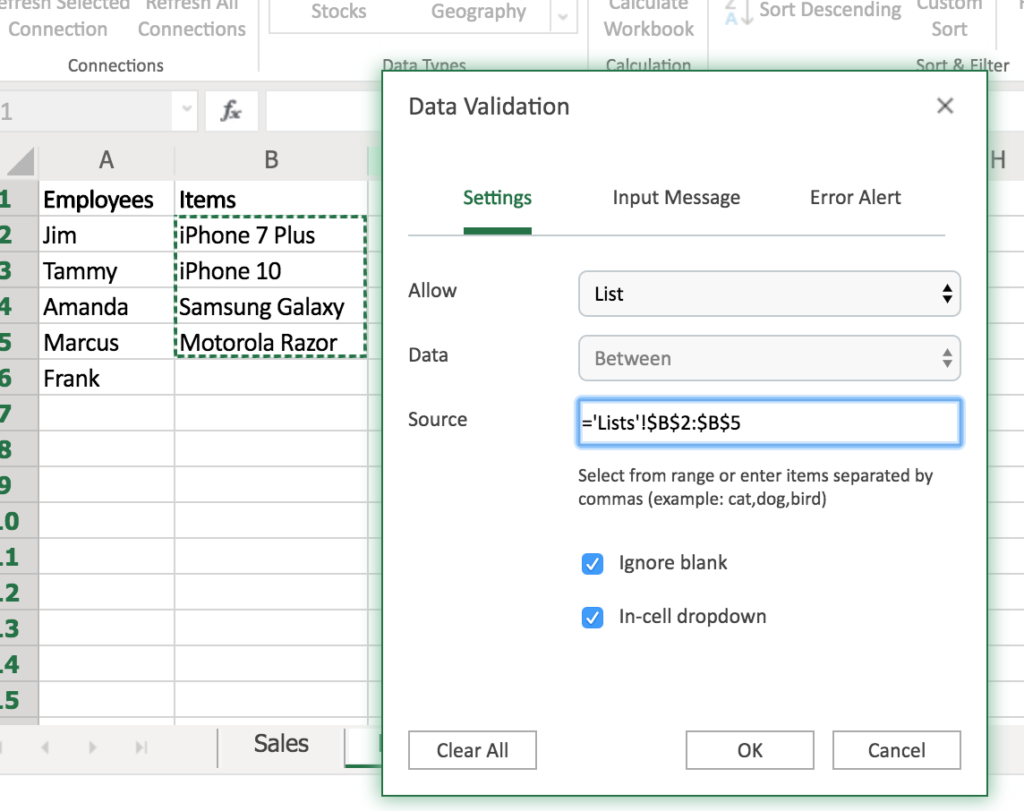
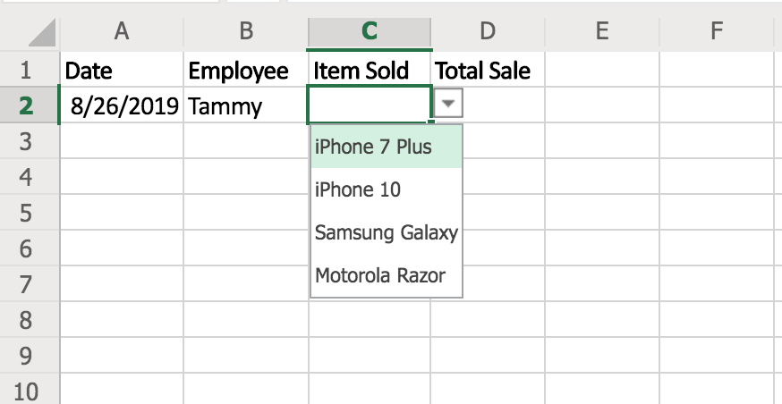
In this example, we will repeat the same steps for our “Item Sold” column, using the “Items” list as our drop-down options.
- (In Sales tab) Click on Column C Header
- Click on Data Validation in the top menu Data option
- Click on List in the Allow drop down
- Click inside the Source input field
- Click on the Lists tab
- Highlight cells B2, B3, B4, and B5
- Press Enter
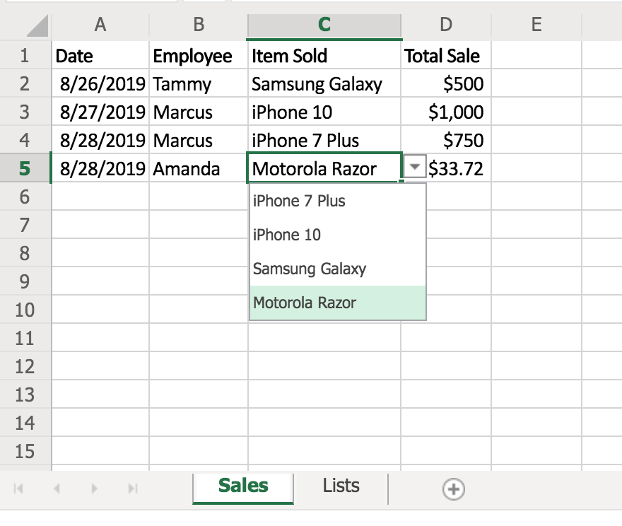
That’s it!
Now you have 2 columns that have 2 separate drop down lists.
What if you only need one cell and not the entire column?
The steps above show you how to add a drop-down list to all cells within the entire column. But if you need to add a drop-down list to only a single cell, the steps are nearly identical!
Instead of clicking on the column header cell, you will only click on the cell you need the drop-down on. For instance, we added the Employees list to the entire Employees column, so we highlighted Cell B Header Cell, then opened up the Data Validation window.
However, if we only needed the first cell to contain the drop-down, then instead of highlighting the entire column by selecting the B Header Cell, we would’ve just selected cell B1, then opened up the Data Validation window and follow the rest of the steps accordingly.
Pretty simple! Comment below if you’re having any difficulties or want help with something more complex!